Indonesian E-commerce App Reviews Sentiment Analysis
Background
Mobile or portable devices are the most widely used technology of this era. With the increase of internet coverage and the pandemic situation, people are getting used to staying indoors and limiting their outdoor activities. This results in increased usage of mobile devices in addition to increased online commerce transactions. Users are free to download and install any e-commerce app to their liking. Their choice, though personal and subjective, were influenced by the players of the e-commerce sector. Businesses are competing to provide better, cheaper, and safer shopping experiences. However, that competition produces an astronomically long list of options for users to choose from. While that’s just a natural implication of competition, users are overwhelmed by those choices. They need a comparison, a simple score, or others’ experience1 to quickly decide which one is the most suitable for their needs.
Businesses will then analyze user reviews to optimize their app or services and to deliver features that are demanded by their users1.
In this post, we’ll do sentiment analysis on Indonesian e-commerce app reviews. The goal of this post is to create a model to classify the review’s sentiment. Sentiments here are classified into two categories, negative and positive sentiment.
Context
For clarity, I will start by defining some recurring terms that are used throughout this analysis.
Sentiment is like a mood or feelings polarity of the user, it indicates whether their mood is negative or positive after using the app. Sentiments can be helpful for business analyst to separate reviews into two distinct groups and do further analysis on each group. So then they can extract much more meaningful information. For example, what most negative reviews are complaining about, or what features do users love the most. That example is of course non-exhaustive because analyses are tailored to the needs of each company.
The polarity of a review can be inferred from the word choices, usage of insults, emotionally expressive emojis, and low rating scores. While this rule is logical from a human perspective, a machine might beg to differ. Since we’re going to do classification analysis, we need a sample of reviews labeled with the ground truth of sentiment polarity. I generated the ground truth based on the rating score, so reviews with ratings 1 and 2 were labeled negative, reviews with ratings 4 and 5 were labeled positive while rating 3 reviews were not included in the sample.
Explanatory Data Analysis
App reviews were scraped from Google Play Store and Apple Store for 9 Indonesian e-commerce apps. Here is the list of the scraped e-commerce reviews:
- Blibli
- Tokopedia
- Shopee
- Bukalapak
- Lazada
- JD.ID
- Zalora
- Bhinneka
- Elevenia
Data fetching is executed periodically using workflow executor, Airflow; here’s an instruction on how to setup Airflow in Docker.
The oldest review dated back to 2015. But the majority of the data are coming from 2021. The total row count from the oldest until the latest fetched by the time writing this is roughly 2.7 million reviews. The image below shows the scraped reviews distribution by year.
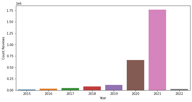
Figure 2.1.1 Scraped Reviews Distribution by Year
Since some e-commerce is more popular than others, the number of reviews fetched will vary. The image below shows the distribution of scraped reviews by e-commerce name.
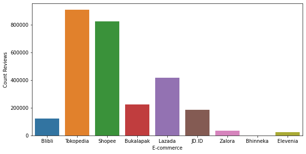
Figure 2.1.2 Scraped Reviews Distribution by App Name
When sampling the data, I didn’t pay any attention to the app distribution because sentiments are not dependent on e-commerce. If a review is negative, it will remain negatively polarized even if it was sent to another app.
However, it is not the case with rating distribution. Due to the ground truth sampling method that I use, I need to make sure that it is unbiased by equally representing each polarity. Hence, I sampled the data stratified by their ratings. So here’s how it looks before and after sampling.
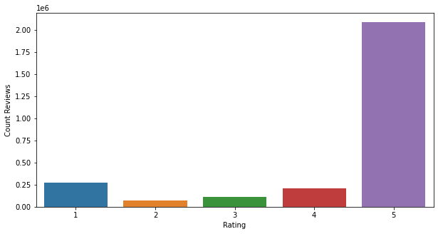
Figure 2.1.3 Scraped Reviews Distribution by Rating
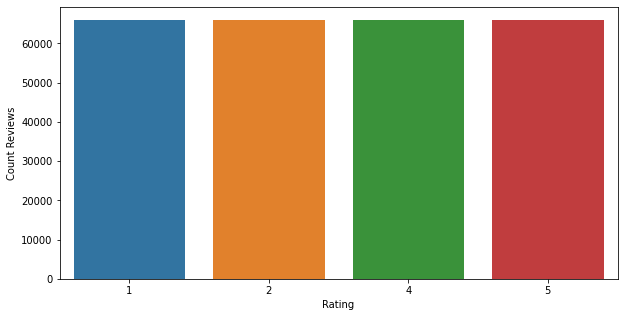
Figure 2.1.4 Sampled Reviews Distribution by Rating
As you can see on the scraped review rating distribution, the total reviews with a rating of 2 are the lowest. The exact value is not visible from the chart, but it’s roughly 66.000 reviews. As to not introduce any bias, I have to sample an equal amount of reviews from each rating score. That’s the reason why I limit the sampled frequency of each group to 66.000.
Then it’s now obvious that the sampled sentiment distribution is exactly 132.000 for negative and 132.000 for positive.
Data Cleaning
As I’ve explained previously, sentiments can be inferred from several factors. However, reviews usually contains a lot of “useless” stuff that didn’t contribute to sentiment polarity. Such as:
- stopwords,
- numbers,
- symbols, and
- HTML code
You might ask, why do I say symbols didn’t contribute to the sentiment polarity. Yes, they did actually. But since symbols can be used on both negative and positive sentiment, not cleaning them will just confuse the algorithm. For example, you could say that the exclamation mark (!) is usually used in negative reviews like “Very slow app!! Cannot log in at all!!”. But it can also be used in positive reviews like this, “Great app, love it!!”. Also, if we include symbols in the datasets, it will only introduce a bias towards certain sentiment that mostly uses that specific symbol, while lowering the confidence of classifying the opposite sentiment.
HTML code is also cleaned, just in case the scraper is experiencing some errors and scraping the code instead of just the text.
While stopwords are also usually cleaned, in my case removing it didn’t produce noticeable or even any improvement whatsoever to the model. I don’t really understand why though. Maybe because the stopwords remover that I use are not doing their job properly or because the model understands that stopwords are useless and thus giving it low weights. Whichever it is, I decided not to remove stopwords because the remover algorithm is quite slow.
Baseline Model: Logistic Regression
When doing analysis using a deep learning model, it is a best practice to train baseline model using traditional machine learning such as logistic regression. There’s not much thought as to why I choose logistic regression here, but from my experience and light research on the web I found out that this algorithm yields the best accuracy for text classification.
The baseline model’s accuracy will be used as a target we need to achieve with the deep learning model. Also, since training machine learning model is significantly faster, I can compare different cleaning methods to use on the deep learning model that will give me better classification power.
For this model preprocessing, I’m using a TF-IDF vectorizer to translate words to numbers that the machine can understand. With 85% accuracy, here are the model evaluation results:
              precision    recall  f1-score   support

           0       0.85      0.84      0.85     33142
           1       0.84      0.85      0.85     32858

    accuracy                           0.85     66000
   macro avg       0.85      0.85      0.85     66000
weighted avg       0.85      0.85      0.85     66000
Long Short-term Memory (LSTM)
First things first, what is LSTM. Long Short-term Memory or LSTM for short, is simply a flavor of Recurrent Neural Network (RNN). Recurrent Neural Network is suitable to be used in Natural Language Processing (NLP) domain, because it can learn the seqeunce and relationship between words2.
Mahendran Venkatachalam from gotensor.com summarizes RNN so beautifully, and I quote:
Recurrent Neural Networks (RNNs) add an interesting twist to basic neural networks. A vanilla neural network takes in a fixed size vector as input which limits its usage in situations that involve a ‘series’ type input with no predertemined size. Whereas RNNs are designed to take a series of input with no predertemined limit on size. - (Vekatachalam, M. 2019)
RNN is a structure that contains loops and allows persistence of information2 by feeding information from all of previous layers in time as inputs for the next layer. But there is a problem with this structure. Can you guess it?
Well, if you are familiar with how neural network improves its network, you’d notice the increase complexity of updating the neuron’s weights3. In vanilla neural network, improvement are propagated from output to input by updating the weights of the previous neuron based on the gradient. But notice that RNN layer chain can grow as long as your series length. This creates a problem called vanishing gradient and also exploding gradient. For more detailed explanation on the vanishing gradient problem, please refer to SuperDataScience (2018) and Or, B. (2020).
But to summarize, vanishing gradient happens because when a neural network is initialized, their weights are randomized. This randomization is not a problem usually, but if your network is very deep then the time to train your model will skyrocket. Gradient in layers closest to the output is probably good enough to update the neuron’s weights and train the layer4. But due to vanishing gradient, the closest to the input layer the gradient will become less and less. Therefore, half of the network layers are not trained properly and don’t forget that this “untrained”4 layer’s output is forwarded to the layer in front of it and so on and finally to the output layer.
The problem of vanishing gradient can be solved by introducing short-term memory in form of “forget gate”, and thus LSTM was born. For detailed explanation on how this so called “gate” works, please refer to Phi, M. (2018).
Moving on, here’s how my layer structure looks like.
Model: "sequential"
_________________________________________________________________
Layer (type)                 Output Shape              Param #
=================================================================
embedding (Embedding)        (None, 120, 100)          4536200
_________________________________________________________________
spatial_dropout1d (SpatialDr (None, 120, 100)          0
_________________________________________________________________
lstm (LSTM)                  (None, 64)                42240
_________________________________________________________________
dense (Dense)                (None, 1)                 65
=================================================================
Total params: 4,578,505
Trainable params: 4,578,505
Non-trainable params: 0
_________________________________________________________________
I used a Word2Vec in the embedding layer, but technically you can swap it out with any other text embedding algorithm. Word2Vec receives word as input and yield floating point numbers to represent that word. It is basically having the same functionality as TF-IDF in the baseline model previously.
After training the model using an Adagrad optimizer, I got this result:
              precision    recall  f1-score   support

           0       0.84      0.85      0.85     26251
           1       0.85      0.84      0.85     26549

    accuracy                           0.85     52800
   macro avg       0.85      0.85      0.85     52800
weighted avg       0.85      0.85      0.85     52800
This LSTM model also has 85% accuracy. As such, there is no improvement from the baseline model.
CNN
CNNs are infamous in the domain of computer vision, because it is specifically designed for processing image inputs. If you want to learn the details of CNN, please refer to Saha, S. (2018), CS231n (n.d.), and Brownlee, J. (2019).
You might think that if it is designed for processing image, it won’t be as good as LSTM then. Well, that design is exactly the reason why CNN is as powerful as LSTM in NLP domain. Let me explain.
For computer vision related topics like image analysis & classification, the network needs to understand and remember certain things such as spatial and temporal dependencies.
Imagine if you train an image classification model on regular neural network. You are forced to flatten the input from a 2D image to 1D values. What’s the problem here? The spatial information of the pixel fed into the network is lost. Therefore the network will have a hard time figuring out the pattern in the data. Now, what if you keep the dimensionality of the input? Then the model will surely be able to learn the pattern much better.
This is exactly what we need in NLP domain as well. Sentences are constructed based on a rule called grammar, and you can’t just rearrange the words because then it will lose its meaning. That’s where the CNN’s spatial dependencies ability comes into play. CNN will remember the structure from your data, and then try to find pattern from it.
Not only that, CNN can also capture temporal dependencies. It can capture the dependencies between a data point and its neighboring data points. Let’s say, a review that has the word “like” will most likely classified as having positive sentiment, right. But what if the full review is actualy “I don’t like this app”. As a human you’ll understand right away that the sentiment is clearly negative. However if the algorithm didn’t remember the temporal dependencies of “don’t” that negates the positive sentiment of the next word, then it won’t be able to correctly classify it.
Also, if you noticed, CNN models will train much faster compared to LSTM. This is true because in case of review data, the length of the input is quite low compared to image input.
Here is how my CNN layer is structured:
Model: "sequential"
_________________________________________________________________
Layer (type)                 Output Shape              Param #
=================================================================
embedding (Embedding)        (None, 475, 100)          6940200
_________________________________________________________________
conv1d (Conv1D)              (None, 238, 128)          64128
_________________________________________________________________
average_pooling1d (AveragePo (None, 119, 128)          0
_________________________________________________________________
conv1d_1 (Conv1D)            (None, 60, 64)            41024
_________________________________________________________________
average_pooling1d_1 (Average (None, 30, 64)            0
_________________________________________________________________
flatten (Flatten)            (None, 1920)              0
_________________________________________________________________
dense (Dense)                (None, 1)                 1921
=================================================================
Total params: 7,047,273
Trainable params: 7,047,273
Non-trainable params: 0
_________________________________________________________________
Training the model using an Adagrad optimizer gave me this result:
              precision    recall  f1-score   support

           0       0.86      0.83      0.85     23800
           1       0.84      0.87      0.85     24200

    accuracy                           0.85     48000
   macro avg       0.85      0.85      0.85     48000
weighted avg       0.85      0.85      0.85     48000
Sadly there is no significant improvement compared to LSTM. However this model has a tendency to classify reviews as positive thus having higher false positive rate and low precision.
CNN Stacking Ensemble
While CNN didn’t produce significant improvement as shown previously, we can improve its score by using ensemble. In this case, I will use stacking ensemble.
To explain it simply, stacking is an ensemble method created by combining several model trained with different parameters. Then their output will be fed into a meta classifier to finally make a classification. Still not simple enough? Don’t worry, here is an illustration to explain it visually.
 Figure 7.1 An example scheme of stacking ensemble learning.5
So here’s how my stacked model looks like:
Model: "model"
__________________________________________________________________________________________________
Layer (type)                    Output Shape         Param #     Connected to
==================================================================================================
input_1 (InputLayer)            [(None, 120)]        0
__________________________________________________________________________________________________
embedding (Embedding)           (None, 120, 100)     4536200     input_1[0][0]
__________________________________________________________________________________________________
conv1d (Conv1D)                 (None, 60, 128)      25728       embedding[0][0]
__________________________________________________________________________________________________
conv1d_1 (Conv1D)               (None, 60, 128)      38528       embedding[0][0]
__________________________________________________________________________________________________
conv1d_2 (Conv1D)               (None, 60, 128)      51328       embedding[0][0]
__________________________________________________________________________________________________
conv1d_3 (Conv1D)               (None, 60, 128)      64128       embedding[0][0]
__________________________________________________________________________________________________
conv1d_4 (Conv1D)               (None, 60, 128)      76928       embedding[0][0]
__________________________________________________________________________________________________
global_max_pooling1d (GlobalMax (None, 128)          0           conv1d[0][0]
__________________________________________________________________________________________________
global_max_pooling1d_1 (GlobalM (None, 128)          0           conv1d_1[0][0]
__________________________________________________________________________________________________
global_max_pooling1d_2 (GlobalM (None, 128)          0           conv1d_2[0][0]
__________________________________________________________________________________________________
global_max_pooling1d_3 (GlobalM (None, 128)          0           conv1d_3[0][0]
__________________________________________________________________________________________________
global_max_pooling1d_4 (GlobalM (None, 128)          0           conv1d_4[0][0]
__________________________________________________________________________________________________
concatenate (Concatenate)       (None, 640)          0           global_max_pooling1d[0][0]
                                                                 global_max_pooling1d_1[0][0]
                                                                 global_max_pooling1d_2[0][0]
                                                                 global_max_pooling1d_3[0][0]
                                                                 global_max_pooling1d_4[0][0]
__________________________________________________________________________________________________
dropout (Dropout)               (None, 640)          0           concatenate[0][0]
__________________________________________________________________________________________________
dense (Dense)                   (None, 128)          82048       dropout[0][0]
__________________________________________________________________________________________________
dropout_1 (Dropout)             (None, 128)          0           dense[0][0]
__________________________________________________________________________________________________
dense_1 (Dense)                 (None, 1)            129         dropout_1[0][0]
==================================================================================================
Total params: 4,875,017
Trainable params: 4,875,017
Non-trainable params: 0
__________________________________________________________________________________________________
It’s quite a big structure, but basically conv1d to conv1d_4 are the level 0 layer. The first dense network is the level 1 layer, and dense_1 network is the output layer with sigmoid activation.
Training this model using an Adagrad optimizer gave me this result:
              precision    recall  f1-score   support

           0       0.86      0.85      0.85     26251
           1       0.86      0.86      0.86     26549

    accuracy                           0.86     52800
   macro avg       0.86      0.86      0.86     52800
weighted avg       0.86      0.86      0.86     52800
We finally see an improvement, even though quite a small one. However, I’m still not satisfied yet. I’m gonna try another ensemble technique on the next section.
Voting Ensemble: Deep Learning + Traditional ML
To satiate my curiosity, I decided to train numerous ML algorithms aside from the baseline logistic regression. The results are an array of models with unique strength and classification power. With some even reached 88% precision in one class. But their scores are all over the place, and there’s no model that is distinctly more superior than others.
Now that I have this collection of models in my hands, let’s do a simple voting ensemble with them.
Voting ensemble is really simple, as the name implies, all we have to do is to choose the class that has the highest support from the classification models. The support is calculated from the classifier models prediction probability. Say a model is predicting that an input has 85% probability of having positive sentiment, that probability is used as a support for classifying that input as positive. The negative support in this case is 15%.
Since different models have different strengths and weaknesses, combining them in this style is beneficial to get the full benefit of their individual strengths while offsetting their weaknesses.
The list below is listing all classifier models, and their respective score, that are used in the voting ensemble.
model                  class  precision    recall  f1-score
===========================================================
LogisticRegression         0       0.85      0.85      0.85
                           1       0.85      0.85      0.85
___________________________________________________________
DecisionTree               0       0.82      0.77      0.79
                           1       0.79      0.83      0.81
___________________________________________________________
RandomForest               0       0.83      0.86      0.84
                           1       0.85      0.82      0.84
___________________________________________________________
SupportVector              0       0.85      0.84      0.84
                           1       0.84      0.85      0.85
___________________________________________________________
NearestCentroid            0       0.67      0.93      0.78
                           1       0.88      0.55      0.68
___________________________________________________________
NaiveBayes                 0       0.82      0.86      0.84
                           1       0.86      0.81      0.83
___________________________________________________________
KNeighbors                 0       0.79      0.37      0.50
                           1       0.59      0.90      0.71
___________________________________________________________
LSTM                       0       0.84      0.85      0.85
                           1       0.85      0.84      0.85
___________________________________________________________
CNN                        0       0.86      0.85      0.85
                           1       0.86      0.86      0.86
___________________________________________________________
Voting ensemble didn’t require fitting because the output is not predicted, but calculated. You still need to train the classifier model though.
Here’s the result of the voting ensemble:
              precision    recall  f1-score   support

           0       0.88      0.91      0.90     33103
           1       0.91      0.88      0.89     32897

    accuracy                           0.89     66000
   macro avg       0.90      0.89      0.89     66000
weighted avg       0.89      0.89      0.89     66000
Right away you may have noticed that the voting ensemble score is better than any of the previous models.
Verdict
Comparing the models based on their F1-score and accuracy shows a clear win for voting ensemble. I’m using F1-score because I want to balance their predictive power of negative and positive sentiment.
Voting also didn’t require training additional classifier, unlike stacking ensemble. Which is great and saves us some more time to do other things.
So, that’s it for this post. After exploring different classification algorithm we came into conclusion that for my dataset of Indonesian app reviews, the best model is built using voting ensemble technique. Having 90% F1-score for negative sentiment, 89% F1-score for positive sentiment, and 89% accuracy.
References
[1] Genc-Nayebi, N., & Abran, A. (2017). A systematic literature review: Opinion mining studies from mobile app store user reviews. Journal of Systems and Software, 125, 207–219. https://doi.org/10.1016/j.jss.2016.11.027
[2] Li, D., & Qian, J. (2016). Text sentiment analysis based on long short-term memory. 2016 1st IEEE International Conference on Computer Communication and the Internet, ICCCI 2016, 471–475. https://doi.org/10.1109/CCI.2016.7778967
[3] Amidi, A., & Amidi, S. (n.d.). Recurrent Neural Networks cheatsheet. Retrieved January 28, 2022, from https://stanford.edu/~shervine/teaching/cs-230/cheatsheet-recurrent-neural-networks [Archived 30 Jan, 2022]
[4] SuperDataScience Team. (2018). Recurrent Neural Networks (RNN) - The Vanishing Gradient Problem. https://www.superdatascience.com/blogs/recurrent-neural-networks-rnn-the-vanishing-gradient-problem [Archived 30 Jan, 2022]
[5] Stacking Ensemble Learning for Short-Term Electricity Consumption Forecasting - Scientific Figure on ResearchGate. Available from: https://www.researchgate.net/figure/An-example-scheme-of-stacking-ensemble-learning_fig3_324552457 [accessed 29 Jan, 2022] [Archived 30 Jan, 2022]
[6] Venkatachalam, M. (2019). Recurrent Neural Networks – Remembering what’s important. https://gotensor.com/2019/02/28/recurrent-neural-networks-remembering-whats-important/ [Archived 30 Jan, 2022]